

Contents
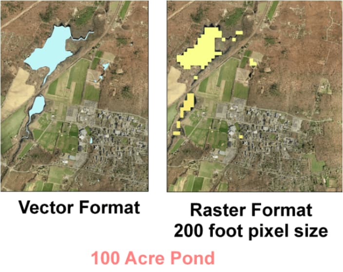
There are two primary types of spatial data—namely raster and vector. Raster data is made up of a grid of pixels; vector data is composed of vertices and paths. Those two types of data are reflected in mapping solutions, as shown below.
Our design challenge was to build faster vector maps. In particular, we needed to overcome performance challenges. Let’s dive into how we did it, using a W’s approach.
What?
In general, the objective of any software performance engineering is to build predictable performance into systems. That is achieved by specifying and analyzing quantitative behavior from the very beginning of a system, through to its deployment and evolution.
In this case, every vector tile request has a 2-step process.
- Request validations and subsequent signed URL generation.
- Redirect to fetch the specified vector tiles with 302 redirection.

When we started, the end-to-end vector maps rendering process took roughly between 800 to 1300 milliseconds, which was too slow and needed improvement.
Where?
By design, the potential latency fix might occur in one of three layers:
- Network layer
- AWS Infra layer
- Application layer
In our context, those layers are represented below:
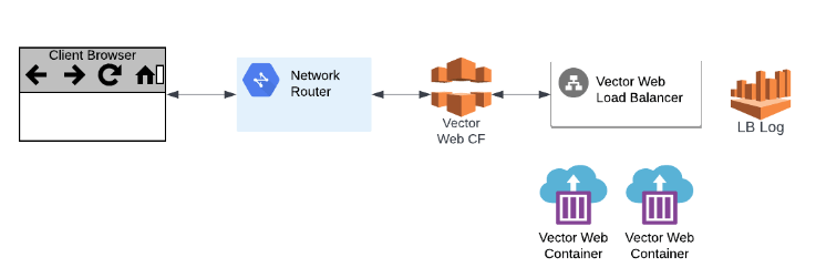
- The Network layer is related to the OSI (Open Systems Interconnection) reference model over the system network.
- AWS Infra layer covers the latency from, to and within AWS components.
- Application layer is directly related to the developers’ code for rendering vector maps.
Why?
As the first step, we targeted the Application layer as it is the most controllable section. After refining a few caching mechanisms and logger usage, the system didn’t gain major performance results. These low-hanging technical solutions didn’t provide much improvement.
On troubleshooting with few instrumentation measures, the big fish is caught at the infrastructure layer.
As depicted above, the application layer is consistently performing with lower 2 digits of milliseconds during multiple experimentation runs/methodologies. But the endpoints between the network and app containers are consuming the major portion of the performance.
How?
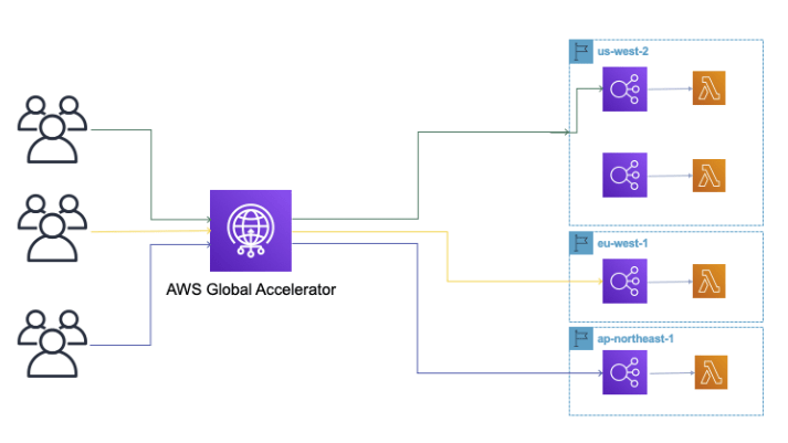
After narrowing down the layer we wanted to improve, we decided to experiment with the modern AWS component (Global Accelerator) as a replacement for AWS cloud front for our performance scenarios.
| Influencing factors | CloudFront | Global Accelerator |
|---|---|---|
| Performance coverage | Improves performance for both static and dynamic HTTP(S) content | Improves performance for a wide range over TCP or UDP |
| Static/dynamic IPs | Uses multiple sets of dynamically changing IP addresses | Leverages a fixed set of 2 static IP addresses |
| Edge Location usage | Uses edge locations to cache the content | Uses edge to find an optimal pathway to nearest endpoint |
AWS global accelerator really gains a huge win on the end-to-end performance with few experimentation cycles. (You can read more about AWS global accelerator in this blog post.)
By design, it is quite logical due to Top-3 infra architectural influencing elements.
Thus, our performance problem is resolved with ~67% gain. Overall, this was a great learning experience that not only improved our vector mapping performance, but also taught us a lot about the value of experimentation.
Share this article: